Walk through a nuclear markers analysis
role=“alert”>This page provides a brief introduction to PickCells via a walkthrough which takes you from the PickCells welcome screen to displaying a histogram to compare nuclear intensities in two different image samples.
Contents
- Treating stem cells with a compound
- Download sample images
- Start PickCells and log in
- Create a new experiment
- Import images
- Explore the MetaModel View
- Identify nuclei
- Compute basic nuclei features
- Visualise nuclei data
- Other explorations
- Where next?
- References
Treating stem cells with a compound
Consider the following hypothesis:
If we treat stem cells with some compound A, then stem cells differentiate.
To test this hypothesis, we can perform the following biological experiment in the lab:
- We culture the cells both with (treated) and without (control) the addition of compound A.
- We wait for enough time for the treatment to potentially have an effect and then we fix the cells and perform immuno-staining for markers of differentiation.
- We then go to our microscope and take several images of both the control and treated conditions. We make multi-channel images so that each channel corresponds to the signal of a specific marker of differentiation.
Here are some example images:
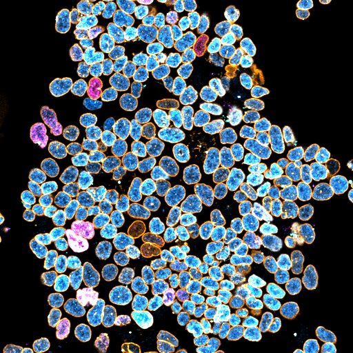
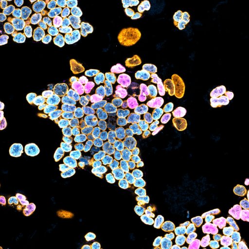
where:
- Magenta highlights Differentation.
- Cyan highlights Stemness.
- Orange highlights the Nucleus Contour.
At this point we could qualitatively assess whether the markers are more expressed in the treated samples versus the control samples just by looking at the images. However, it is not always clear by eye whether a difference truly exists and, more importantly, we may miss sub-visual patterns that only quantification at the single cell level can reveal.
So, to quantify the level of differentiation with single cell resolution, we can create a PickCells experiment to conduct the following tasks:
- Image analysis: a. Load all colour images. b. Identify the nuclei in all images. c. Compute the average or integrated intensity within each nucleus for all channels i.e. for each marker of differentiation.
- Data analysis: a. View a histogram of nuclear intensities. b. Compare the intensities between the control and treated conditions.
How we use PickCells to carry out these tasks is now described.
Download sample images
Download the sample images archive file <a href=https://datasync.ed.ac.uk/index.php/s/VdTV5V5PmEWDc07/download?path=%2FSampleDatasets&files=Nuclear_Markers_Analysis.tar.gz" target="_blank">Nuclear_Markers_Analysis.tar.gz (password ‘pickcells’)
Unpack the contents of the .tar.gz file.
This creates a folder called Nuclear_Markers_Analysis/. This folder contains both raw and segmented images for both control and treated samples:
Readme.md

./color_images:
Ctrl_1.ics
Ctrl_1.ids
Ctrl_2.ics
Ctrl_2.ids
Treated_1.ics
Treated_1.ids
Treated_2.ics
Treated_2.ids

./segmented_images:
Ctrl_1_nuclei.ics
Ctrl_1_nuclei.ids
Ctrl_2_nuclei.ics
Ctrl_2_nuclei.ids
Treated_1_nuclei.ics
Treated_1_nuclei.ids
Treated_2_nuclei.ics
Treated_2_nuclei.ids
Start PickCells and log in
Start PickCells.
Once PickCells has started, click Log in.
If you have not logged in before, the New User… dialog will appear:
- Enter a User name, password, and then confirm your password.
- Click Login.
If you have already logged in before, the Login dialog will appear:
- Enter your user name and password.
- Click Login.
The user screen will appear.
Create a new experiment
To create a new experiment, click the Create a new experiment icon, located on the right-hand side in the My Experiments panel.
The Experiment Wizard will appear:
- Enter a Name for the experiment: NuclearMarkers
- Click Browse… to open up a file browser.
- Browse to a location where you want to hold your experiment database folders.
- Click the Create new folder icon:

- Enter a name for the new folder: PickCellsExperiments
- Click the new folder.
- Click Open
- The path to your new folder should now be in the Location field.
- Enter a short Description about the experiment: This is a nuclear markers analysis.
- Click OK.
A new database will be created on your file system, in PickCellsExperiments/, which will be reopened every time you load this experiment. In this example, the database folder has name NuclearMarkers/.
Your experiment will now be visible on the user screen:
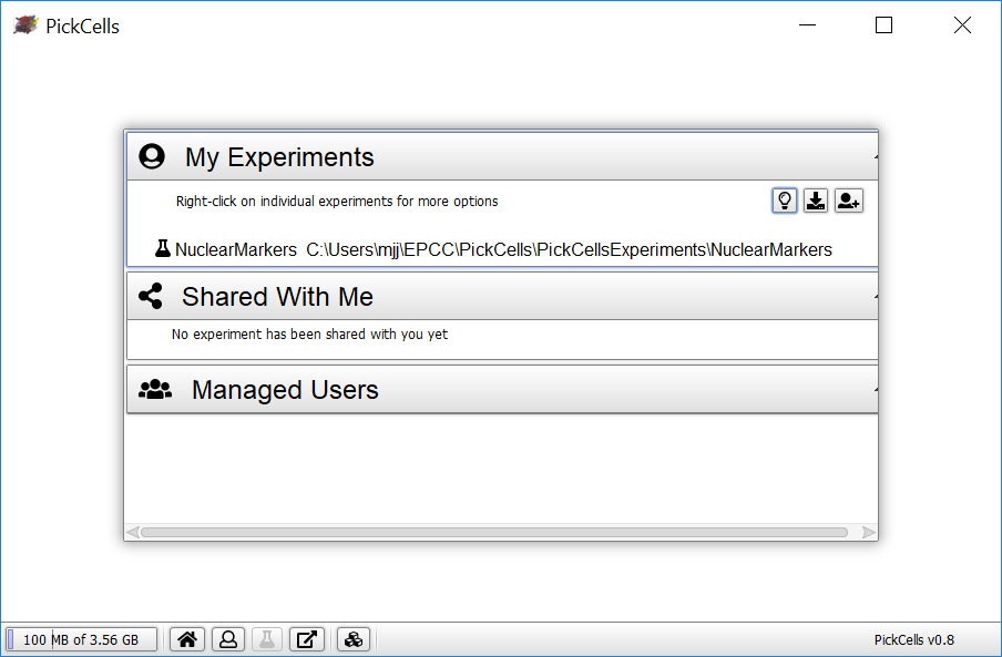
Now, load your experiment:
- Right-click on the experiment name, NuclearMarkers.
- Select Load.
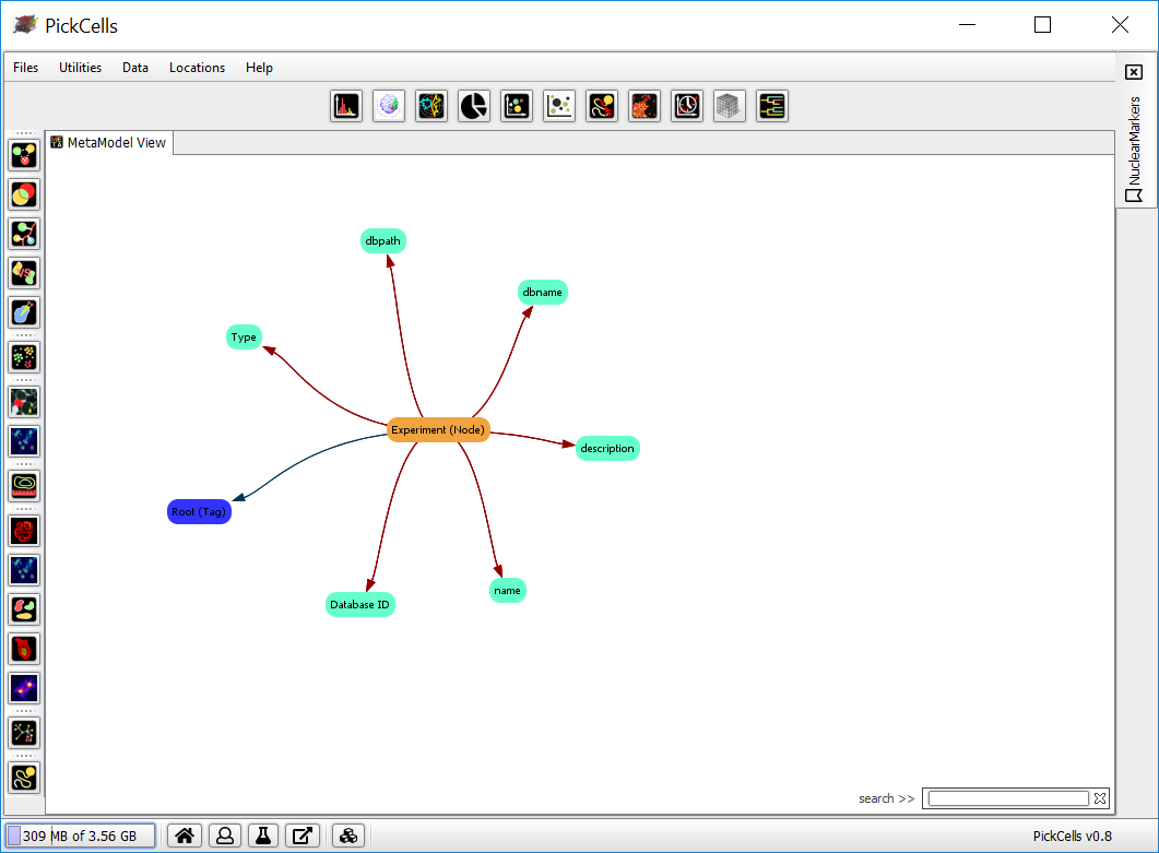
A new workbench, with the experiment’s MetaModel View, will appear.
Import images
To import images, select Files => Import… => Colour Images.
This opens the import dialog.
You now need to select the images to import. The dialog offers two options:
- Add Library: Library files are commonly created by microscopy software and contain a collection of images. Common examples include Leica
.lifand Zeiss.lsmfiles. This option allows you to select a library file, see the images it contains, then select which of the images you want to import. - Add Images: This option allows you to select image files held within a folder on your file system.
We want to load images, so click Add Images.
A file browser will appear:
- Browse to the folder
Nuclear_Markers_Analysis/color_images/. - Select all the
icsfiles. To select only these files, hold down the Ctrl key and click eachicsfile. - Click Choose.
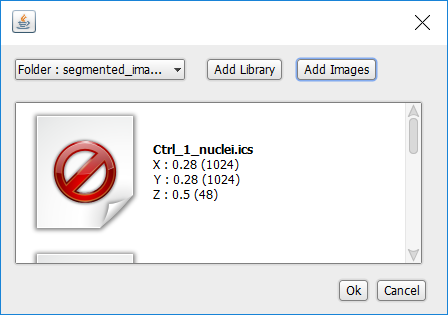
Once you have selected the images to load, a selected images dialog will display a thumbnail and a short description of each selected image.
Click OK.
Enter channel names and colours
The channel names dialog will appear which allows you, for each channel in the images, to select the following:
- Name: A name for the channel. Typically this will be the name of the protein strained for.
- LUT: A colour scheme for the channel. LUT stands for Lookup Table which defines a range of shades for a specific colour.
Enter the following Name values for each channel:
- Channel 0: Differentiation
- Channel 1: Stemness
- Channel 2: Nuclear Envelope
- Channel 3: Golgi
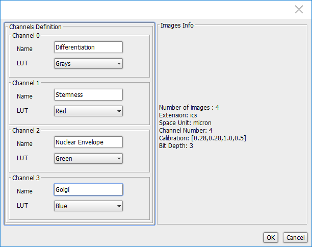
When you are done, click OK.
Wait for PickCells to import images
PickCells will import your selected images and a progress bar will appear while it does so.
To open your experiment’s database folder, select Locations => Database Folder
This folder will contain one .ics and one .ids file for each imported image.
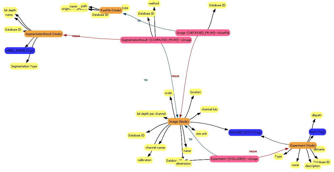
When the images have been imported, the MetaModel View will update with objects representing the images.
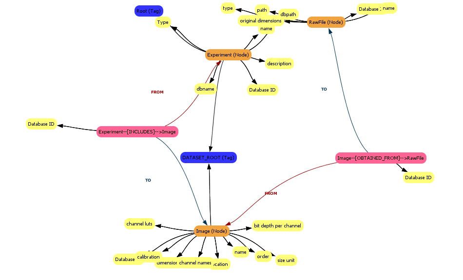
Explore the MetaModel View
Click on an object (a node) to centre the view on that object.
Right-click on an object to open a popup menu which allows you to get more information about the object or to delete the object. For example:
- Right-click on Experiment (Node) and select Show Count. A dialog will appear stating that ‘There are currently 1 Experiment’.
- Right-click on Image (Node) and select Show Count. A dialog will appear stating that ‘There are currently 4 Image’.
- Right-click on Image (Node) and select Table Set. A dialog will appear showing a table with 4 rows, one for each image, with metadata about the images that were loaded. This will include the channel names you entered earlier.
Identify nuclei
One of the most critical steps in image analysis is the accurate identification of the objects that need to be analysed 1 2. This step, termed image segmentation, consists of generating an image where each individual object is given a unique colour:
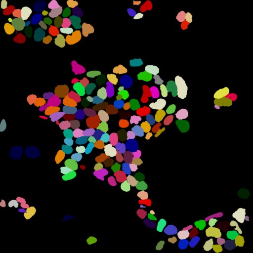
In PickCells, each unique colour provides a unique ID to each object allowing PickCells to identify features, such as shape, position or intensities.
For segmentation, PickCells offers two options:
- Segment images using NESSys (Nuclear Envelope Segmentation System) segmentation module, if you want to do segmentation from within PickCells.
- Import segmented images, if the segmentation modules available in PickCells aren’t suitable for your needs, or you have generated segmentation results using other tools.
We have segmented images, in Nuclear_Markers_Analysis/segmented_images/, so we’ll import these.
Import segmented images
Import the segmented images:
- Select Files => Import… => Segmented Images.
- The steps to select segmented images to import are the same as already described in Select images to import, except that the channel names dialog will not appear.
- Segmented images are in the folder
Nuclear_Markers_Analysis/segmented_images/.
PickCells will check that the segmented images you import have the same dimensions as the colour images you have already imported.
When the images have been imported, the MetaModel View will update with metadata about the segmentation results (look for the Segmentation Result object).
Compute basic nuclei features
Once the segmentation images have been imported, we can create objects with the type of our choice, using the Intrinsic Features module.
To open the Intrinsic Features module, click the Intrinsic Features icon in the vertical toolbar: ![]()
The Intrinsic Features dialog will appear.
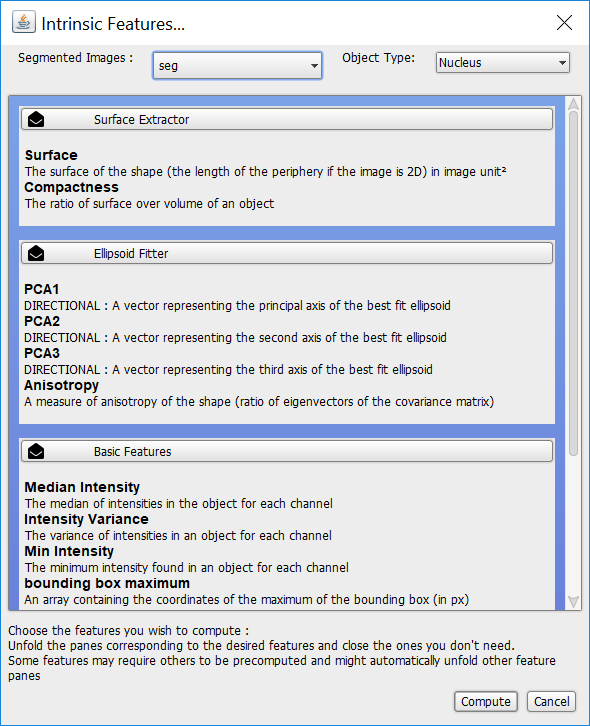
By default we can compute features on our segmented images, ‘seg’, creating a new object type, ‘Nucleus’, to record those features.
There are three classes of features that can be computed:
- Surface Extractor: surface-related features e.g. the surface itsemf or the ratio of surface to volume.
- Ellipsoid Fitter: ellipsoids e.g. a vector representing the principal axis of the best fit ellipsoid.
- Basic Features: intensities, bounding boxes, and volumes.
Recall from earlier that we want to Compute the average or integrated intensity within each nucleus for all channels i.e. for each marker of differentiation., so we will use Basic Features:
- Click Surface Extractor and Ellipsoid Filter so that their panels are closed.
- Click Basic Features so that its panel is open.
The dialog should look like:
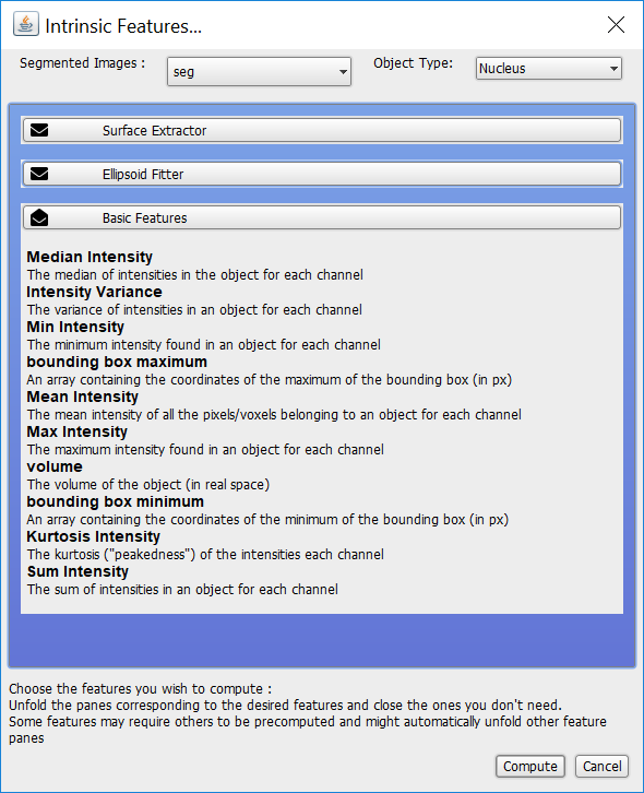
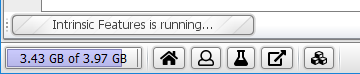
Now, click Compute.
The Intrinsic Features module will start to calculate the basic features, indicated via a progress bar in the bottom-left of the workbench:
When complete, the MetaModel View will update to show the new Nucleus object, ‘Nucleus (Node)’, which has the computed features as properties:
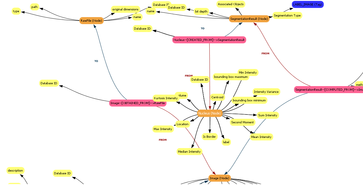
Remember, you can click on Nucleus to centre the MetaModel View on that object, and use right-click to open a popup menu which allows you to get more information about the object.
Visualise nuclei data
Visualisation modules allow us to display data within PickCells. In our example, recall that we have stained for differentiation and stemness markers so we’ll create histograms to view the distribution of the level of ‘differentiation’ and the level of ‘stemness’.
Display all nuclei intensities
To create a new histogram, click the Histogram icon in the horizontal toolbar: ![]()
A Histogram panel will appear. It will be empty as it has no data.
To select data to plot in the histogram, click the Change Data Set icon in the histogram panel’s horizontal toolbar: .
The Dataset Builder dialog will appear. On the left of the Dataset Builder dialog will be a MetaModel Browsing panel, for example:
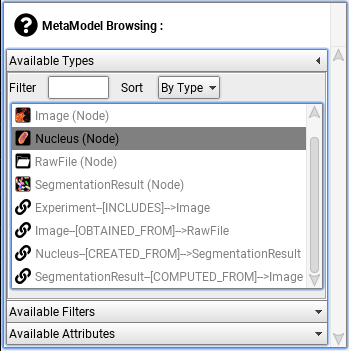
These are objects whose data can be visualised within a histogram.
To select nuclei-related data:
- Select Nucleus (Node) in the MetaModel Browsing panel.
- Click Change, next to the Target Type field, on the right of the Dataset Builder dialog.
- Click Done at the bottom of the Dataset Builder dialog.
The histogram will still be empty but the axes labels will change to ‘Dataset loaded, No dimensions defined’.
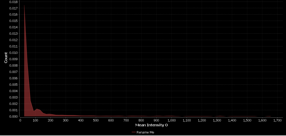
Now, we need to select the ‘dimension’ (i.e. property) to plot. First, plot the mean intensity per nucleus in channel 0, the differentiation marker:
- Click the Change Dimensions icon,

- From the Select a Dimension drop-down list, select Mean Intensity 0
- Click OK
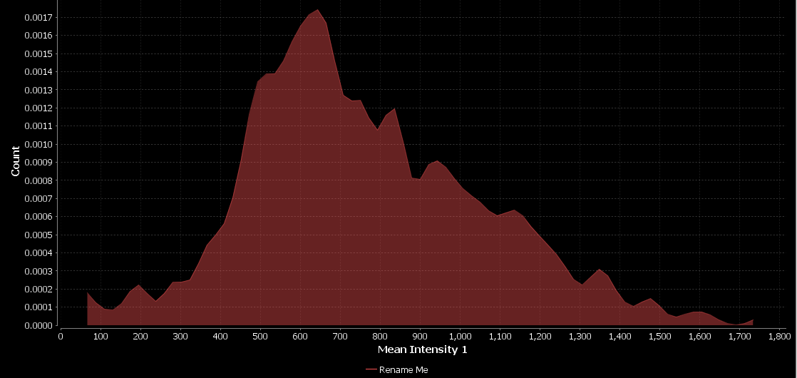
Now, let’s repeat the above, but this time create a new histogram which plots the mean intensity per nucleus in channel 1, the stemness marker:
- Click the Histogram icon in the horizontal toolbar.
- Click the Change Data Set icon in the histogram panel’s horizontal toolbar: .
- Select Nucleus (Node) in the MetaModel Browsing panel.
- Click Change, next to the Target Type field, on the right of the Dataset Builder dialog.
- Click Done at the bottom of the Dataset Builder dialog.
- Click the Change Dimensions icon.
- From the Select a Dimension drop-down list, select Mean Intensity 1
- Click OK
Compare nuclei intensities between conditions
Recall that our goal is to compare distributions between the control and treated conditions. In order to do this, we will group our images by these conditions and then group nuclei based on the image group they belong to.
1. Create filters for control and treated images
First, we use the names of our images as a means of selecting which images have our control conditions (images with ‘Ctrl’ in their name) and which images have our treated conditions (images with ‘Treated’ in their name). To select these images we can use a ‘filter’.
To create a new filter, select Data => New Filter.
The Custom Filter dialog will appear. This allows us to choose the object for which we want to create a filter.
- Select Image (Node)
- Click OK
The Type of Filter dialog will appear with two options:
- Create a filter based on node attributes (properties)
- Create a filter based on node connections (relationships)
The name of the image is a property (or attribute) of the image so:
- Select Create a filter based on node attributes.
- Click Next
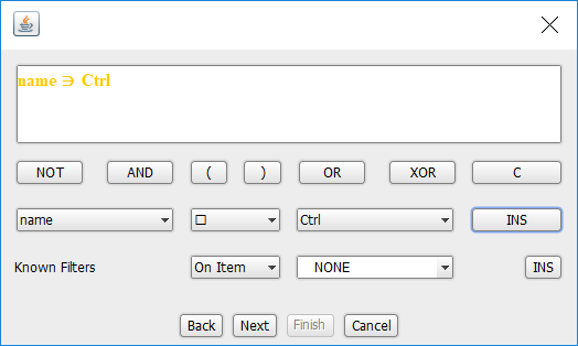
The query builder dialog will appear which allows us to define how the filter operates. We want our filter to accept an image if its ‘name’ attribute contains the string ‘Ctrl’:
- From the drop-down list on the left of the dialog, select Item attribute
- From the Please select a key list, select name
- Click OK
- From the drop-down list on the right of the dialog, select Constant
- In the Value Selector dialog, enter Ctrl
- Click OK
- Click INS (Insert)
The query builder should look like the following:
Now:
- Click Next
- Enter a name for the filter: Control
- Click in the Short Description area
- Click Finish
Now, repeat the above and create a filter called ‘Treated’ that filters Image objects that have the name ‘Treated’ in their ‘name’ property.
2. Create a dataset which groups nuclei based on the whether they in are control or treated images
Now, instead of visualising data from all nuclei objects, we will use a ‘path’ (introduced in What kind of data can I generate?) to select the nuclei objects to visualise based on the results of the filter.
Click the Histogram icon in the horizontal toolbar.
Click the Change Data Set icon in the histogram panel’s horizontal toolbar: .
First, we will find all paths between Image objects and Nucleus objects. To request that the Dataset Builder search for paths between these nodes:
- In the Search Strategy panel, select Create a Path
- In the Metamodel browsing panel, select Image (Node)
- In the Path Definition’s Start block, double-click on the ‘?’ (question mark)
The ‘?’ should be replaced by a small Image icon.
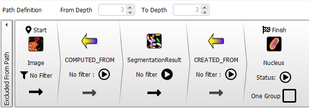
- In the Metamodel browsing panel, select Nucleus (Node)
- In the Path Definition’s Finish block, double-click on the ‘?’ (question mark)
The ‘?’ should be replaced by a small Nucleus icon and the Path Definition should expand, and appear as follows:
Now, we use our new image filter to group paths from Image nodes to Nucleus nodes into two categories - Control and Treated - so the targets of the paths (i.e. the Nucleus nodes) are also grouped into these two categories.
To apply the filter, right-click on the arrow within the Image element in the Path Definition’s Start block, and select Split here.
The Path Splitting panel will expand. This panel allows us to define how we want to group the objects that have been found, thereby splitting the path. We want to split Nucleus nodes by the Control and Treated categories, so:
- In the Path Splitting panel, select Split in 2.
- In the MetaModel Browsing panel, click Available Filters to expand the Available Filters panel.
- Select the Control filter.
- Click Change
- In the Filter Combination panel, enter the following values:
- Accepted: Control
- Rejected: Treated
Here, we are assuming that any image whose name does not contain the string ‘Ctrl’ is assumed to be a treated image. As we have only control and treated images this is a reasonable assumption, in this case.
Finally, rename the dataset:
- In the My DataSet panel, right-click Rename Me…
- Enter: “Control and Treated”.
The Dataset Builder should look like this:
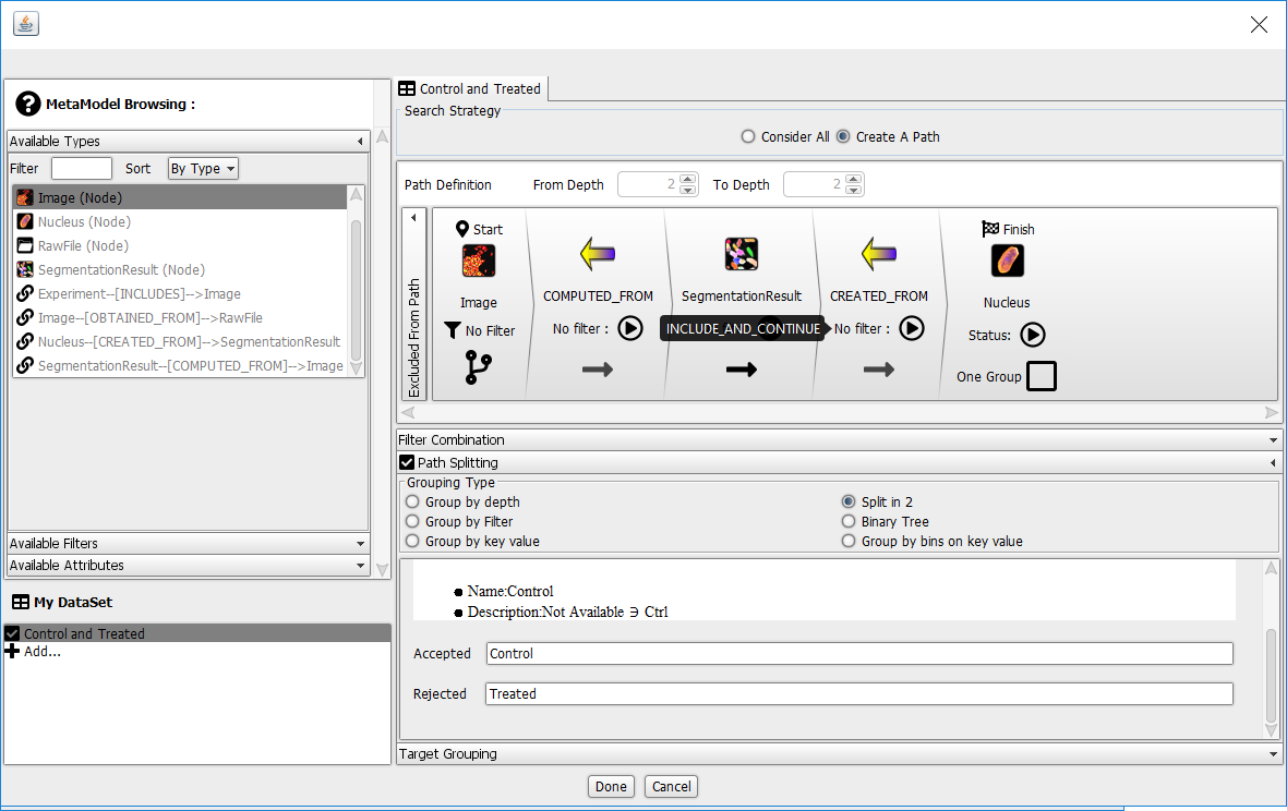
Click Done at the bottom of the Dataset Builder dialog.
We have now created a dataset which only contains the Nucleus nodes associated with the Control images.
We can now plot the level of nuclear intensities in each of the conditions:
- Click the Change Dimensions icon,
- From the Select a Dimension drop-down list, select Mean Intensity 0.
- Click OK
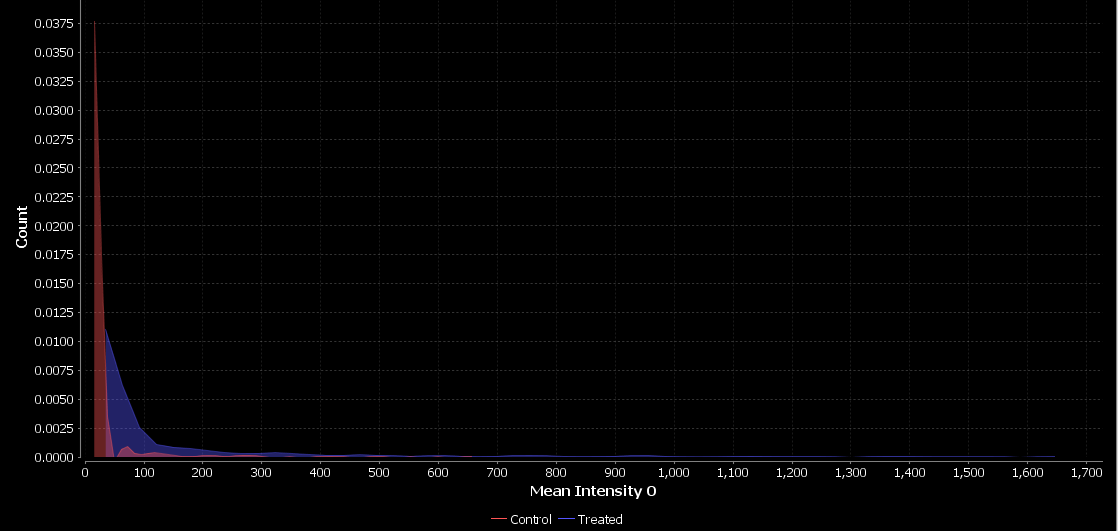
Here, we observe a small shift in intensity in the treated condition which may indicate that the treatment does induce differentiation in these cells.
Other explorations
There is much more that could be done within this experiment in order to identify more complex patterns in the data or simply to validate that there are no biases in the analysis. Here are a few ideas that you could try with this experiment:
- Create nuclei categories by setting a threshold on the level of differentiation marker e.g. phenotype: differentiated vs. non differentiated.
- View nuclei categories with an image overlay, to validate by eye the nuclei categories created with the thresholding technique.
- Display a pie chart to compare control vs. treated conditions and view percentages.
Where next?
This walkthrough only covers a small fraction of what can be done with PickCells. You could now:
- Check out the tutorials demonstrating other features of PickCells.
- See the features supported by PickCells.
- Look at the How To category on the PickCells Colony forum.